Multiple Series Pattern Causality Analysis: Unveiling System-Wide Interactions
Stavros Stavroglou, Athanasios Pantelous, Hui Wang
Source:vignettes/matrix.Rmd
matrix.RmdThis vignette provides a comprehensive demonstration of multivariate pattern causality analysis, a powerful technique for investigating complex interactions within large-scale systems. This approach is particularly useful when dealing with multiple interconnected time series, allowing us to move beyond pairwise analysis and understand system-wide dynamics. The key aspects of this analysis include:
- Matrix-based causality assessment: Quantifying causal relationships between all pairs of time series in the system, represented in a matrix format.
- System-wide pattern identification: Identifying recurring patterns of behavior across the entire system, revealing underlying dynamics.
- Visualization of complex causal relationships: Using graphical representations to make intricate causal networks more understandable.
- Analysis of effects across the entire system: Measuring the overall impact of causality within the system, providing insights into the collective behavior.
The matrix-based approach is particularly well-suited for the study of:
- Financial market networks: Analyzing the interconnectedness of stock prices and other financial instruments.
- Economic systems: Understanding the relationships between various economic indicators and their impact on the overall economy.
- Social networks: Investigating the spread of information and influence within social structures.
- Complex ecological systems: Studying the interactions between different species and environmental factors.
Pattern Causality Matrix
In this vignette, we will utilize the DJS dataset, which comprises 29 stock price series. This dataset provides a sufficiently large and complex system to demonstrate the capabilities of our multivariate pattern causality analysis.
library(patterncausality)
data(DJS)
#head(DJS)
Before estimating the causality matrix, it is crucial to determine
the optimal parameters for our analysis. These parameters, including the
embedding dimension (E) and time delay (tau),
significantly influence the accuracy and reliability of the results. We
use the optimalParametersSearch function to identify these
optimal values:
dataset <- DJS[,-1] # remove the date column
params <- optimalParametersSearch(
  Emax = 3,
  tauMax = 3,
  metric = "euclidean",
  dataset = dataset,
  verbose = FALSE
)
print(params)
With the optimal parameters identified, we can now estimate the
pattern causality matrix using the pcMatrix function. This
function calculates the causality between all pairs of time series in
the dataset, resulting in a matrix representation of the system’s causal
structure.
result <- pcMatrix(
  dataset = dataset,
  E = 3,           # Embedding dimension
  tau = 1,         # Time delay
  metric = "euclidean",
  h = 1,           # Prediction horizon
  weighted = FALSE  # Unweighted analysis
)
The resulting analysis yields three matrices, each representing a
different aspect of causality: positive, negative, and dark causality.
These matrices can be accessed through the pc_matrix
object.
print(result)
#> Pattern Causality Matrix Analysis:
#>
#> Number of items: 29
#>
#> Positive causality matrix:
#>                        X3M American.Express     Apple    Boeing
#> X3M                     NA        0.2261268 0.2224979 0.2565688
#> American.Express 0.2318415               NA 0.2198748 0.2522231
#> Apple            0.2283262        0.2680412        NA 0.2622407
#> Boeing           0.2507485        0.2711864 0.2869058        NA
#> Caterpillar      0.2330168        0.2438080 0.2966432 0.3024545
#>                  Caterpillar
#> X3M                0.2549020
#> American.Express   0.2511664
#> Apple              0.2674617
#> Boeing             0.2675737
#> Caterpillar               NA
#> ...
#>
#> Negative causality matrix:
#>                        X3M American.Express     Apple    Boeing
#> X3M                     NA        0.2421696 0.2406948 0.2295209
#> American.Express 0.2523844               NA 0.2480438 0.2174616
#> Apple            0.2592275        0.2353952        NA 0.2456432
#> Boeing           0.2649701        0.2397094 0.2243536        NA
#> Caterpillar      0.2556611        0.2291022 0.2209212 0.2019002
#>                  Caterpillar
#> X3M                0.2405732
#> American.Express   0.2192846
#> Apple              0.2248722
#> Boeing             0.2290249
#> Caterpillar               NA
#> ...
#>
#> Dark causality matrix:
#>                        X3M American.Express     Apple    Boeing
#> X3M                     NA        0.5317036 0.5368073 0.5139104
#> American.Express 0.5157740               NA 0.5320814 0.5303153
#> Apple            0.5124464        0.4965636        NA 0.4921162
#> Boeing           0.4842814        0.4891041 0.4887406        NA
#> Caterpillar      0.5113221        0.5270898 0.4824356 0.4956453
#>                  Caterpillar
#> X3M                0.5045249
#> American.Express   0.5295490
#> Apple              0.5076661
#> Boeing             0.5034014
#> Caterpillar               NA
#> ...
The plot function for object pc_matrix
provides a powerful tool for visualizing these complex matrices. By
plotting each causality type separately, we can gain a deeper
understanding of the system’s dynamics.
- Positive causality status
plot(result, "positive")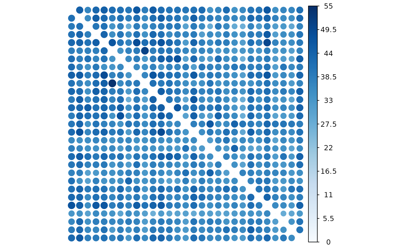
- Negative causality status
plot(result, "negative")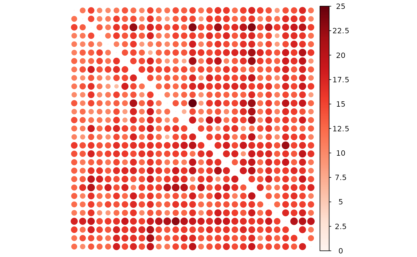
- Dark causality status
plot(result, "dark")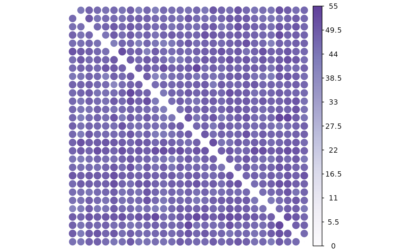
The visualization reveals a clear positive connection within the system, indicating a tendency for stocks to influence each other positively.
Pattern Causality Effect
Following the matrix calculation, we can quantify the total effect
within the system using the pcEffect function. This
function aggregates the causality measures to provide a system-wide
perspective on the overall impact of pattern causality.
effects <- pcEffect(result)
print(effects)
#> Pattern Causality Effect Analysis
#> --------------------------------
#>
#> Positive Causality Effects:
#>                     received exerted   Diff
#> X3M                   650.70  634.25  16.45
#> American.Express      630.98  650.71 -19.72
#> Apple                 661.12  660.70   0.42
#> Boeing                688.59  688.43   0.15
#> Caterpillar           701.02  682.44  18.58
#> Chevron               650.07  635.85  14.22
#> Cisco.Systems         579.50  632.94 -53.44
#> Coca.Cola             634.74  627.41   7.34
#> DowDuPont             668.46  668.23   0.23
#> ExxonMobil            612.87  591.98  20.88
#> General.Electric      623.13  622.74   0.39
#> Goldman.Sachs         599.67  662.85 -63.18
#> IBM                   669.13  634.43  34.70
#> Intel                 640.67  626.83  13.84
#> Johnson...Johnson     647.65  601.69  45.96
#> JPMorgan.Chase        600.89  615.90 -15.01
#> McDonald.s            653.29  662.28  -8.99
#> Merck                 608.59  645.31 -36.72
#> Microsoft             615.45  605.13  10.32
#> Nike                  652.96  679.98 -27.02
#> Pfizer                605.23  605.80  -0.57
#> Procter...Gamble      620.69  570.01  50.67
#> The.Home.Depot        636.16  682.05 -45.89
#> Travelers             613.74  581.12  32.62
#> United.Technologies   625.72  664.30 -38.58
#> UnitedHealth.Group    621.44  637.87 -16.43
#> Verizon               630.72  623.24   7.48
#> Walmart               669.86  594.11  75.75
#> Walt.Disney           643.93  668.38 -24.45
#>
#> Negative Causality Effects:
#>                     received exerted   Diff
#> X3M                   719.26  729.68 -10.41
#> American.Express      712.08  700.91  11.17
#> Apple                 707.09  687.52  19.57
#> Boeing                703.02  676.41  26.60
#> Caterpillar           678.31  676.03   2.28
#> Chevron               715.89  737.31 -21.42
#> Cisco.Systems         752.02  724.54  27.48
#> Coca.Cola             712.08  759.47 -47.40
#> DowDuPont             712.68  674.83  37.85
#> ExxonMobil            748.99  767.41 -18.42
#> General.Electric      678.39  734.08 -55.69
#> Goldman.Sachs         792.84  689.82 103.02
#> IBM                   706.97  731.20 -24.23
#> Intel                 723.44  705.11  18.33
#> Johnson...Johnson     724.40  743.30 -18.90
#> JPMorgan.Chase        735.29  734.19   1.10
#> McDonald.s            694.97  716.52 -21.56
#> Merck                 739.65  709.82  29.83
#> Microsoft             719.92  762.08 -42.16
#> Nike                  717.16  654.36  62.80
#> Pfizer                711.68  739.91 -28.23
#> Procter...Gamble      715.60  815.15 -99.54
#> The.Home.Depot        734.57  662.25  72.32
#> Travelers             734.16  780.05 -45.89
#> United.Technologies   741.72  708.36  33.35
#> UnitedHealth.Group    735.82  714.69  21.13
#> Verizon               744.45  730.70  13.74
#> Walmart               693.07  760.45 -67.38
#> Walt.Disney           692.26  671.61  20.65
#>
#> Dark Causality Effects:
#>                     received exerted   Diff
#> X3M                  1430.04 1436.07  -6.03
#> American.Express     1456.93 1448.38   8.55
#> Apple                1431.79 1451.78 -19.99
#> Boeing               1408.40 1435.15 -26.75
#> Caterpillar          1420.67 1441.54 -20.87
#> Chevron              1434.04 1426.84   7.20
#> Cisco.Systems        1468.48 1442.52  25.97
#> Coca.Cola            1453.18 1413.12  40.06
#> DowDuPont            1418.86 1456.95 -38.08
#> ExxonMobil           1438.15 1440.61  -2.46
#> General.Electric     1498.48 1443.18  55.30
#> Goldman.Sachs        1407.49 1447.33 -39.84
#> IBM                  1423.91 1434.37 -10.47
#> Intel                1435.88 1468.06 -32.17
#> Johnson...Johnson    1427.95 1455.01 -27.06
#> JPMorgan.Chase       1463.82 1449.91  13.91
#> McDonald.s           1451.75 1421.20  30.55
#> Merck                1451.75 1444.87   6.89
#> Microsoft            1464.63 1432.79  31.84
#> Nike                 1429.88 1465.66 -35.78
#> Pfizer               1483.09 1454.29  28.80
#> Procter...Gamble     1463.71 1414.84  48.87
#> The.Home.Depot       1429.27 1455.70 -26.43
#> Travelers            1452.10 1438.83  13.27
#> United.Technologies  1432.56 1427.34   5.22
#> UnitedHealth.Group   1442.74 1447.44  -4.70
#> Verizon              1424.83 1446.06 -21.22
#> Walmart              1437.07 1445.44  -8.37
#> Walt.Disney          1463.81 1460.01   3.80
The total effect of pattern causality can be observed, providing a measure of the overall strength of causal interactions within the system.
- Positive causality status
plot(effects, status="positive")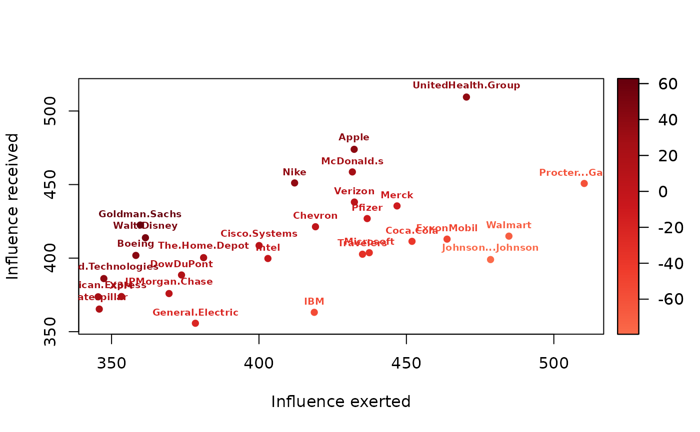
- Negative causality status
plot(effects, status="negative")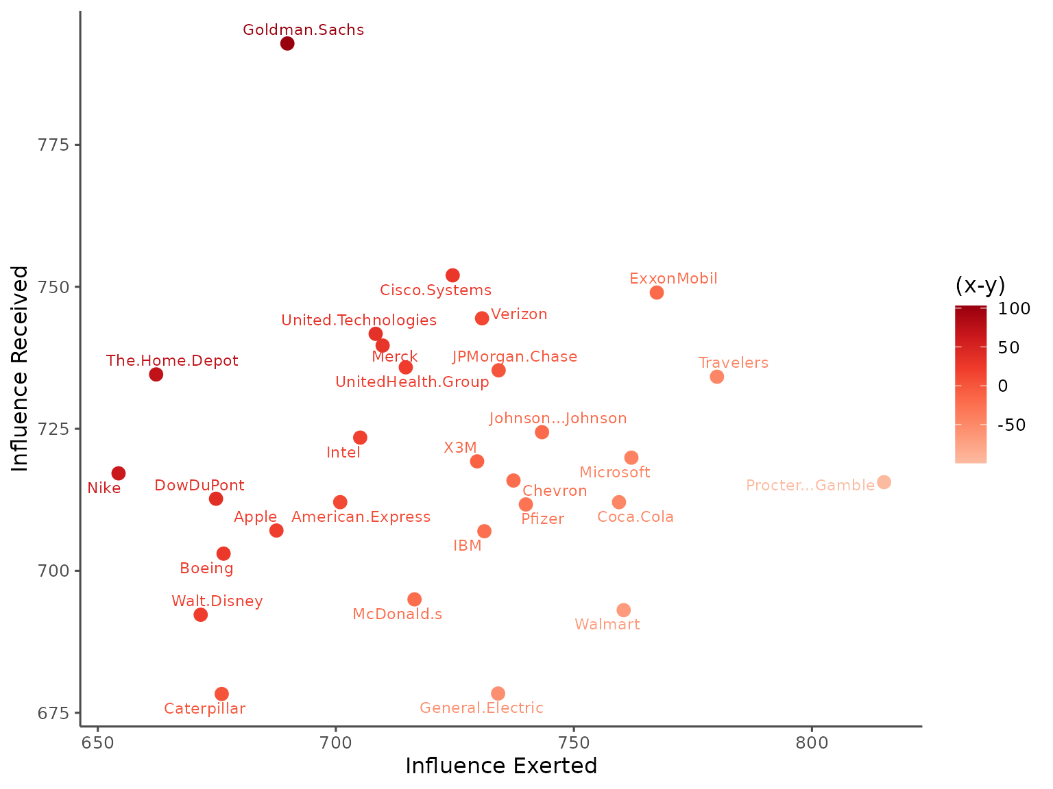
- Dark causality status
plot(effects, status="dark")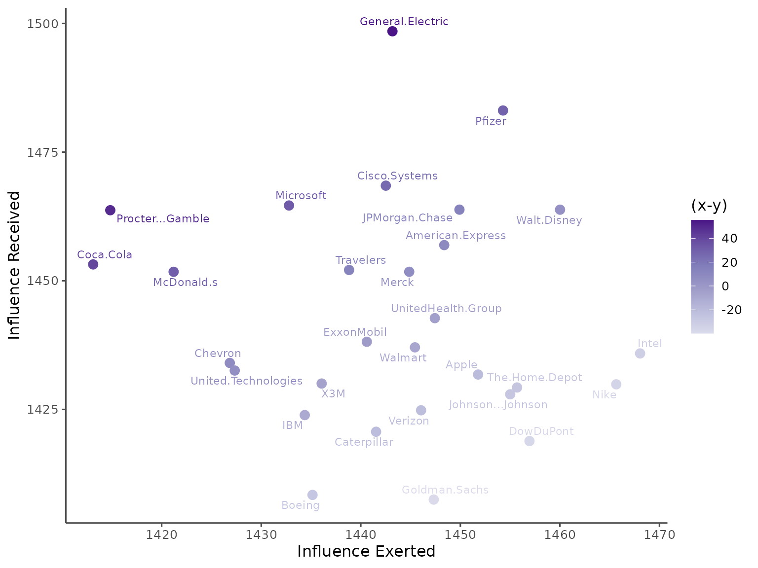
Cross Matrix analysis
Sometimes, we also need to face the problem that X has multiple
series, and Y also has multiple series, we want to know the causality
between each series in X and each series in Y, to save the computation
time, we can use the pcCrossMatrix function to get the
causality matrix from each series in X to Y.
This time we construct the datasets for X and Y in stock dataset.
dataset <- DJS[, -1]

X <- dataset[, 1:10]
Y <- dataset[, 11:29]
Then we can estimate the causality matrix from each series in X to Y and give the new matrix from X to Y.
result_cross <- pcCrossMatrix(
  X = X,
  Y = Y,
  E = 3,
  tau = 1,
  metric = "euclidean",
  h = 1,
  weighted = FALSE,
  verbose = FALSE
)
The new matrix will be saved in the result_cross object,
we can also plot the matrix by the plot function.
plot(result_cross, "positive")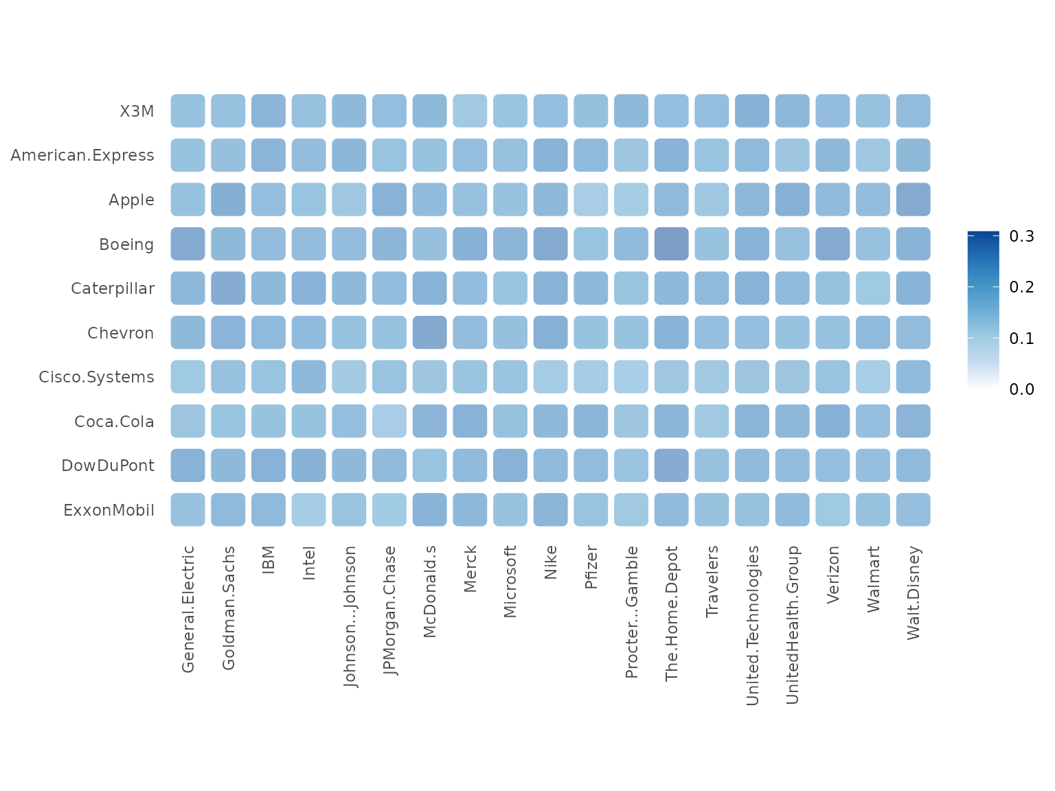
This will show the causality matrix from each series in X to Y and the color of the matrix represents the causality strength in the whole period.
We provide the multiple types of multi-series pattern causality analysis here and it would be useful to face many different situatiuons for the matrix analysis and network analysis.