Analyzes pattern causality matrices to compute and summarize the directional effects of different causality types (positive, negative, dark) between system components.
Value
An object of class "pc_effect" containing:
positive: Data frame of positive causality effects
negative: Data frame of negative causality effects
dark: Data frame of dark causality effects
items: Vector of component names
summary: Summary statistics for each causality type
Details
Calculate Pattern Causality Effect Analysis
The function performs these key steps:
Processes raw causality matrices
Computes received and exerted influence for each component
Calculates net causality effect (difference between received and exerted)
Normalizes results to percentage scale
Related Packages
vars: Vector autoregression for multivariate time series
lmtest: Testing linear regression models
causality: Causality testing and modeling
See also
pcMatrix for generating causality matrices
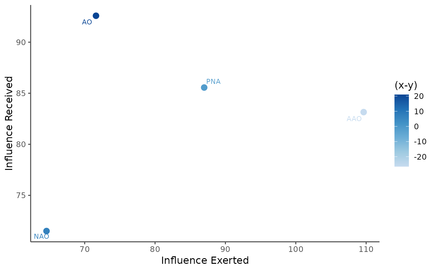
plot.pc_effect for visualizing causality effects
Examples
# \donttest{
data(climate_indices)
dataset <- climate_indices[, -1]
pcmatrix <- pcMatrix(dataset, E = 3, tau = 1,
                    metric = "euclidean", h = 1,
                    weighted = TRUE)
effects <- pcEffect(pcmatrix)
print(effects)
#> Pattern Causality Effect Analysis
#> --------------------------------
#>
#> Positive Causality Effects:
#>     received exerted   Diff
#> AO    131.66  113.90  17.76
#> AAO   111.69  140.63 -28.94
#> NAO   112.86  131.79 -18.93
#> PNA   140.90  110.80  30.11
#>
#> Negative Causality Effects:
#>     received exerted   Diff
#> AO     28.02   35.74  -7.73
#> AAO    44.05   33.40  10.65
#> NAO    39.64   31.94   7.71
#> PNA    27.06   37.70 -10.64
#>
#> Dark Causality Effects:
#>     received exerted   Diff
#> AO    140.32  150.36 -10.04
#> AAO   144.26  125.97  18.29
#> NAO   147.50  136.27  11.23
#> PNA   132.03  151.50 -19.47
#>
plot(effects)

# }
# }